Graphing Linear Equations With Tables: A Step‑by‑Step Guide
Understanding how to graph linear equations is a fundamental skill in algebra. While many textbooks jump straight to plotting points on a coordinate plane, graphing linear equations with tables offers a clear, systematic approach that reinforces the relationship between variables. This method is especially helpful for visual learners and for students who need a concrete way to see how changes in one variable affect the other.
Why Use a Table Before You Plot?
Creating a table forces you to calculate several ordered pairs, which provides a reliable set of points for the graph. When you learn how to generate these pairs, you gain confidence in the equation’s slope and y‑intercept. A table also serves as a reference for checking work, making it easier to spot errors before you draw the final line.
Step 1 – Identify the Equation’s Form
Most introductory problems present a linear equation in one of three common forms: standard form (Ax + By = C), slope‑intercept form (y = mx + b), or point‑slope form (y – y₁ = m(x – x₁)). Recognizing the form helps you decide which variable to solve for when you build your table. For example, if the equation is already in slope‑intercept form, you can quickly read the slope (m) and y‑intercept (b) and choose convenient x‑values.
Step 2 – Choose a Set of X‑Values
Pick a range of x‑values that includes the y‑intercept and extends a few units in both directions. A typical choice is -3, -2, -1, 0, 1, 2, 3. Selecting values that are easy to calculate reduces the chance of arithmetic mistakes and makes the table easier to read.
Step 3 – Solve for Y Using the Equation
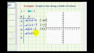
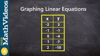
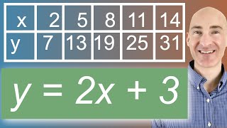
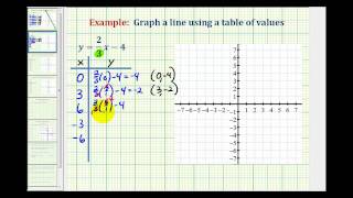
Substitute each x‑value into the equation and solve for y. Record the results in a two‑column table: one column for x and one for y. This is where the phrase Learn how to write a clear, organized table becomes essential. For instance, if the equation is y = 2x + 1, the table would look like this:
- x = -3 → y = -5
- x = -2 → y = -3
- x = -1 → y = -1
- x = 0 → y = 1
- x = 1 → y = 3
- x = 2 → y = 5
- x = 3 → y = 7