How To Vlookup: A Complete Guide for Excel Users
If you work with data in Microsoft Excel, you’ve probably heard the term VLOOKUP. It’s a powerful function that lets you retrieve information from one table and display it in another, saving you countless hours of manual searching. This article walks you through how to Vlookup step by step, from the basic syntax to advanced tips for pulling data across multiple workbooks.
What Is VLOOKUP and When Should You Use It?
VLOOKUP stands for “vertical lookup.” It searches for a value in the first column of a range and returns a value from the same row in a column you specify. Use VLOOKUP when you need to:
- Match product codes to descriptions.
- Combine sales figures from separate sheets.
- Pull a column of data into an Excel report from another spreadsheet using a common identifier.
In Excel, use VLOOKUP whenever your data is organized vertically and you have a unique key (like an ID number) that links tables together.
Basic VLOOKUP Syntax
The function follows this structure:
=VLOOKUP(lookup_value, table_array, col_index_num, [range_lookup])Where:
- lookup_value – The value you want to find.
- table_array – The range containing both the lookup column and the return column.
- col_index_num – The column number (starting at 1) from which to return the result.
- range_lookup – OPTIONAL. FALSE for an exact match, TRUE for an approximate match.
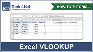
Example: =VLOOKUP(A2, Sheet2!$A$1:$D$500, 3, FALSE) looks for the value in cell A2 on Sheet2, then returns the third column from the matching row.
Step‑By‑Step Tutorial: Learn How to Use VLOOKUP
In this step‑by‑step tutorial, learn how to use VLOOKUP to join two data sets. Follow the numbered steps below:
- Prepare your tables. Ensure the lookup column (e.g., “Employee ID”) is the leftmost column in the source range.
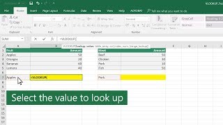
- Enter the formula. Click the cell where you want the result and type =VLOOKUP(.
- Select the lookup value. Click the cell containing the ID you’re searching for, then add a comma.