How To Vlookup In Excel: A Complete Step-by-Step Guide
If you've ever needed to pull specific data from a large spreadsheet, VLOOKUP is one of the most powerful tools available in MS Excel. Whether you're a beginner or looking to sharpen your skills, learning how to use the VLOOKUP function can save you hours of manual searching and data entry.
This guide will walk you through everything you need to know about VLOOKUP Excel, including how the function works, practical examples, and tips to avoid common mistakes.
What Is VLOOKUP In Excel?
VLOOKUP stands for "Vertical Lookup." It is a built-in function in MS Excel that allows you to search for a value in the first column of a table and return a corresponding value from a specified column in the same row.
In simple terms, think of VLOOKUP as a tool that helps you find a piece of information in one column and retrieve related data from another column. This is especially useful when you're working with large datasets and need to match information between two different sources.
The VLOOKUP Syntax Explained
Before you learn how to use the VLOOKUP function, it's important to understand its syntax. Here's the formula structure:
=VLOOKUP(lookup_value, table_array, col_index_num, [range_lookup])
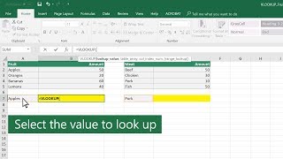
- lookup_value – This is the value you want to search for. It could be a number, text, or a cell reference.
- table_array – This is the range of cells that contains the data you want to search through. The first column of this range should contain the lookup values.
- col_index_num – This is the column number (starting from 1) in the table array from which you want to retrieve the result.
- [range_lookup] – This optional argument determines whether you want an exact match or an approximate match. Use FALSE for an exact match and TRUE (or leave it blank) for an approximate match.
How To Use VLOOKUP In Excel: Step-by-Step
In this section, you will learn about a simple, practical example of how to use VLOOKUP in Excel. Follow these steps carefully.
Step 1: Set Up Your Data
Create two columns of data in your spreadsheet. For example, in the first sheet, list employee IDs in column A and employee names in column B. In another area, you might have a list of employee IDs and need to retrieve the corresponding names.
Step 2: Click On The Cell Where You Want The Result
Select the cell where you want the VLOOKUP formula to display the result. This is typically a cell in a new column or a different section of your worksheet.
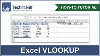
Step 3: Enter The VLOOKUP Formula
Type the following formula:
=VLOOKUP(D2, A2:B10, 2, FALSE)
Here's what this formula does:
- D2 is the cell containing the employee ID you want to look up.
- A2:B10 is the range that contains your data table.
- 2 means you want to return the value from the second column (employee names).
- FALSE ensures you get an exact match for the employee ID.
Step 4: Press Enter